
Winning the Search Task with A Different Geometry
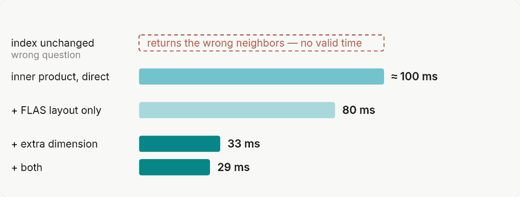
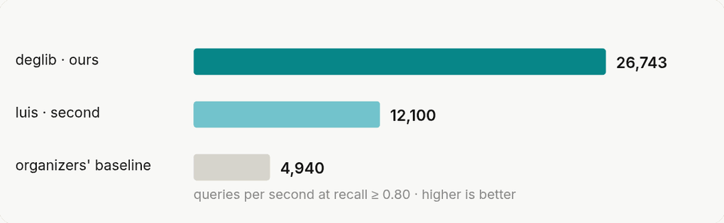
The search task of the SISAP 2026 Indexing Challenge asks for the largest inner products — a notion of similarity our index does not use. Restoring the geometry it is built for, and laying the vectors out for the memory system, took the query batch from about 100 milliseconds to 29 and the submission to first place at 26,743 queries per second.

The SISAP Indexing Challenge is an open competition for similarity search: the organizers set the datasets, every submission is run under the same conditions, and time is only counted above a fixed accuracy. Our overview of this year’s challenge covers all three tasks and how the field came out. This one is about the task we won.
What we entered with is the Dynamic Exploration Graph, the index behind our own search. We have written about it here before, in Dynamic Exploration Graph: Fast Search in Evolving Catalogs — the post to read first if the terms below are new, since it explains what a proximity graph is and why ours is built to absorb insertions and deletions while it is being searched. The open source implementation is deglib, and that is what both submissions are built on.
One thing all tasks have in common: approximate nearest neighbor search trades a small amount of accuracy for a large gain in speed, so every task sets a minimum for that accuracy and measures time second. The measure is recall: the share of the true nearest neighbors a search actually finds. At a recall of 0.80, eight of ten items are true nearest neighbors, and no submission can buy speed by returning worse ones.
What the task asks
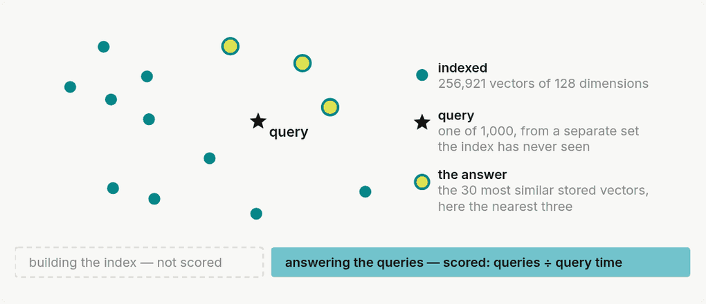
Task 2 stores 256,921 feature vectors of 128 dimensions taken from the interior of Llama-3-8B. For each query vector it asks which 30 stored vectors have the largest inner product with it. The queries are a separate set produced by the same model, but they are not part of the stored collection, and the index is built once and then only answers queries, which is why the task scores query time alone.
What the task does not let us keep is our definition of similarity. Our index ranks by Euclidean distance: the shorter the line between two vectors, the more similar they are. Because we normalize our embeddings to unit length, that ranking is identical to cosine similarity and to the inner product, which is what most embedding models are trained for. Here the vectors are not normalized, and the three come apart.
The picture below shows how. Distance is read off the rings around the query: whichever candidate sits on the innermost ring wins. Cosine similarity throws the lengths away and leaves the angle, which picks the same candidate. The inner product keeps the lengths, and it measures something else: how far a vector reaches along the query’s direction. Its level sets are lines perpendicular to the query rather than rings around it, so a long vector pointing somewhat off can reach past a short one pointing straight at it. One thing the order does not depend on is the length of the query itself: scaling the query stretches every inner product by the same factor.
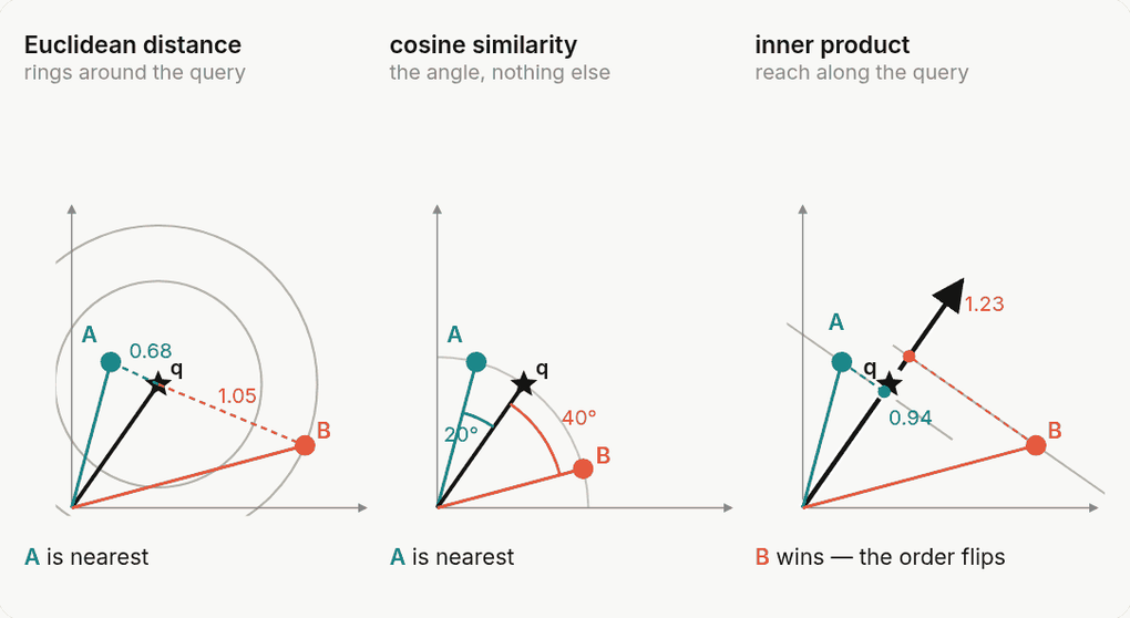
So the starting point was not “our index is slow at this task” but “our index answers a different question”. Run unchanged on these vectors, it returns neighbors that are close, but not the ones the task asks for.
Rank by the inner product directly
The direct fix is to let the graph rank candidates by inner product instead of distance. That works, and it is worth understanding why: the graph still connects vectors that point in similar directions, so a search that walks along its edges still ends up in the right region. What it loses is the guarantee. A proximity graph is navigable because of the triangle inequality: a neighbor of a neighbor cannot be arbitrarily far away, so a greedy walk keeps improving and can stop early. The inner product gives no such bound, so the walk has no reliable signal that it is done, and the only way to reach the required recall is to let it explore much more of the graph. In our own parameter sweeps that meant roughly three times the search budget, and about 100 milliseconds for the query batch.
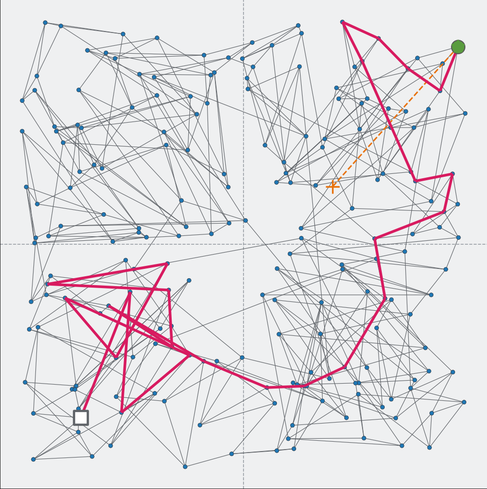
Put the problem back into Euclidean space
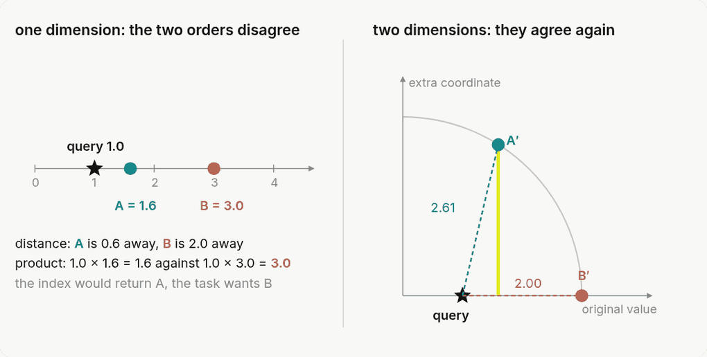
Instead of giving up the geometry, we restore it. Every stored vector gets one extra coordinate, filled up so that all stored vectors end up with the same length; the query gets a zero in that position, which leaves its inner product with every stored vector unchanged. Once all stored vectors are the same length, the expanded distance between a query and a vector is two constants minus their inner product — so the nearest vector is the largest inner product, and an index that ranks by distance answers the task’s question without being told. In the challenge data that turns 128 dimensions into 129. The transformation is not ours: it goes back to Bachrach et al. (2014) and Neyshabur and Srebro (2015), and what made it pay here was combining it with a graph built for Euclidean distance.
It is easiest to see with one-dimensional vectors, where the inner product is simply the product of two numbers and the extra coordinate turns a line into a plane.
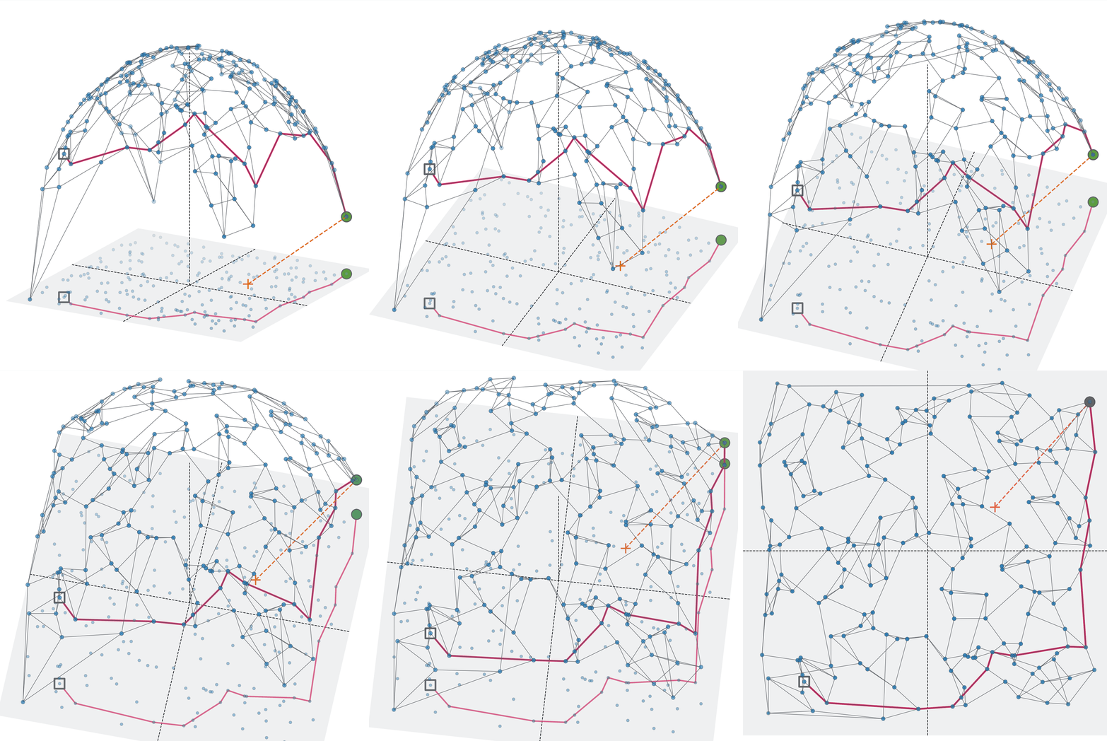
To illustrate the effect, we apply this technique to add a third dimension to the previous two-dimensional example: Constructing the graph on the three-dimensional vectors and the Euclidean distance, we restore the graph’s navigability properties.
Lay the vectors out for the memory system
The remaining gain came from somewhere else entirely. Graph search is limited by memory bandwidth rather than arithmetic: each hop follows pointers to neighbors that may sit anywhere in RAM, and the processor waits for them. FLAS, a sorting method originally published for laying out image grids, arranges the vectors so that similar ones end up next to each other in memory before the graph is built, so a hop usually lands in data that has already been fetched. The order of the two steps decides what each one is worth. On the original geometry the layout alone takes a fifth off the query time, and the extra dimension alone takes two thirds off; applied afterwards to the transformed geometry, the layout is good for another twelve percent. Together they are the difference between about a hundred milliseconds for the batch and twenty-nine.
The result
Against the field, the two steps together are what put the submission in front.
Key Takeaways: Adapting Without Rebuilding
Neither step is a new index. The extra coordinate is a preprocessing pass over the vectors, the layout is a permutation of them before the graph is built, and everything after that is the index we already run — which is what makes both of them portable to a system that is already in production. By combining clever geometric transformations with memory-optimized data layouts, we not only adapted to a new metric but also dominated in query speed, ensuring our customers experience lightning-fast search results, even with highly complex data.
The other task we entered needed the opposite kind of work — not a different geometry, but a cheaper distance computation, because there the time to build the index counts toward the score: two bits per dimension, and why we still rerank.
References
Our submission paper: Hezel, Barthel, Schilling, Schall, Moelle and Jung, Fast and Efficient Approximate Nearest Neighbor Search for High-Dimensional LLM Embeddings (arXiv:2607.20957), with the full method and all measurements.
Our code: Visual-Computing/sisap26-deglib, the submissions for both tasks.
The challenge: SISAP 2026 Indexing Challenge, tasks and datasets, and the leaderboard with every team’s results.
The index itself: our earlier post Dynamic Exploration Graph: Fast Search in Evolving Catalogs.
The conference: SISAP 2026, the 19th International Conference on Similarity Search and Applications, Brno, 14–16 October 2026.
Related Posts

Time to Celebrate! First Place in Vector Search at the SISAP 2026 Indexing Challenge
